Get started with deep learning using Tensorflow 2.0

This is a transcript of the tech talk presented by Usha Rengaraju at Git Commit Show 2020.
- About the speaker
- Use case 1 - Output prediction
- Use case 2 - Fashion image classification
- Use case 3 - Rock paper scissor game
- Questions and answers
- Conclusion
About the speaker
Usha Rengaraju is the first female Indian Kaggle grandmaster. She is the lead at Women in Machine Learning and Data Science (both Bengaluru and Mysore chapters). She is also the organizer of the Tensorflow Users Group Mysore and GDG Mysore.
Traditional programming is the concept of providing machines with data and rules to get answers. Machine Learning is the concept where we feed the machine the data and answers and the machine tells us the rules.
In this hands-on session, we'll be making three ML models for three different use cases using TensorFlow.
Use case 1 - Output prediction
So, we have tabular data for 2 variables (input and output) and then we run our model to predict outputs for a given input. Following is the sample data.
| x | -1 | 0 | 1 | 2 | 3 | 4 |
| y | -2 | 1 | 4 | 7 | 10 | 13 |
First, go to this Google Colab notebook, and in the file section, click on "Save a copy in Drive". A copy of the code will be created in your Drive. You can edit that and follow along with the rest of the blog.
The procedure to make an ML model is
- Import the required libraries
- Define and Compile the Neural Network
- Provide data
- Train the model
We start by importing the required libraries for the project by running the following code
import tensorflow as tf
import numpy as np
from tensorflow import keras
We then create the simplest possible neural network that has 1 layer and that layer has one neuron.
model = tf.keras.Sequential([keras.layers.Dense(units=1, input_shape=[1])])Then we execute the above code to compile the model. The model will map the input x to the output y. Initially, the model is fed with random data and henceforth, there can be some errors. A loss function measures these errors and helps us understand how far we are from accurate predictions.
model.compile(optimizer='sgd', loss='mean_squared_error')Here, the loss is the loss function and the optimizer is what regulates the loss function.
Next up we'll feed in some data. In this case, we are taking 6 xs and 6ys. You can see that the relationship between these is that y=2x-1, so where x = -1, y=-3 etc.
A Python library called Numpy provides lots of array-type data structures that are a defacto standard way of doing it. We declare that we want to use these by specifying the values as an np.array[]
xs = np.array([-1.0, 0.0, 1.0, 2.0, 3.0, 4.0], dtype=float)
ys = np.array([-2.0, 1.0, 4.0, 7.0, 10.0, 13.0], dtype=float)
Now, we fit the data to the model by using the model.fit function. We keep the epochs value to 500 which means the model will map the value 500 times.
model.fit(xs, ys, epochs=500)After the model has been trained, we feed in some sample values to the model to predict the output for us.
Let's say we gave the input as 10 using the model.predict function.
#Input
model.fit(xs, ys, epochs=500)

#Output
#[[30.998993]]
If we observe the data closely, the relationship between X and Y is Y=3X+1, so for input x=10, we should get output 31, right? But with only 6 data points, we can't know for sure if the relationship is correct. As a result, the output for 10 is very close to 31, but not exactly 31.
Use case 2 - Fashion image classification
Let's say we have a set of multiple fashion items like shoes, t-shirts, handbags, etc. The model learns from the data set, and it has to make a prediction for the given input.
You can access the code on this Google Colab notebook.
We start by importing the necessary libraries
# TensorFlow and tf.keras
import tensorflow as tf
from tensorflow import keras

# Helper libraries
import numpy as np
import matplotlib.pyplot as plt

print(tf.__version__)
The fashion mnist is a popular dataset of 70000 images in the keras library. To include the dataset, we run the following code.
fashion_mnist = keras.datasets.fashion_mnist

(train_images, train_labels), (test_images, test_labels) = fashion_mnist.load_data()
We divide the dataset of 70000 images into two categories
| (train_images, train_labels) | (test_images, test_labels) |
|---|---|
| 60000 images | 10000 images |
So, out of 70k images, we used 10k images as test data set.
A label is what is mapped to an image. Basically, we will be predicting the label for our image using the ML model.
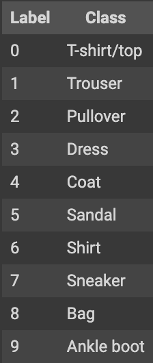
Each image is mapped to a single label. Since the class names are not included with the dataset, store them here to use later when plotting the images.
class_names = ['T-shirt/top', 'Trouser', 'Pullover', 'Dress', 'Coat',
               'Sandal', 'Shirt', 'Sneaker', 'Bag', 'Ankle boot']
We then preprocess the data,. If we inspect the first image in the training set, we see that the pixel values fall in the range of 0 to 255:
plt.figure()
plt.imshow(train_images[0])
plt.colorbar()
plt.grid(False)
plt.show()

#train_images[0] means the first image in the dataset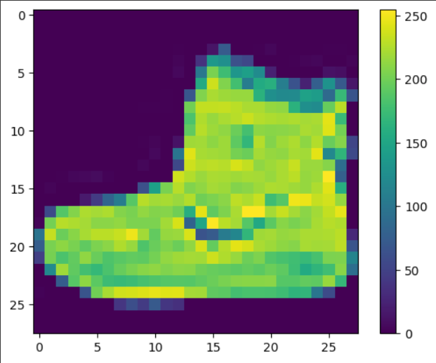
We scale these values to a range of 0 to 1 before feeding them to the neural network model. To do so, divide the values by 255. It's important that the training set and the testing set be preprocessed in the same way:
train_images = train_images / 255.0

test_images = test_images / 255.0
We scale this because the value of a pixel can range from 0-255, and to easily train the model, we scale it down to a value between 0 and 1. This process is called normalization.
To verify that the data is in the correct format and that we're ready to build and train the network, let's display the first 25 images from the training set and display the class name below each image.
plt.figure(figsize=(10,10))
for i in range(25):
    plt.subplot(5,5,i+1)
    plt.xticks([])
    plt.yticks([])
    plt.grid(False)
    plt.imshow(train_images[i], cmap=plt.cm.binary)
    plt.xlabel(class_names[train_labels[i]])
plt.show()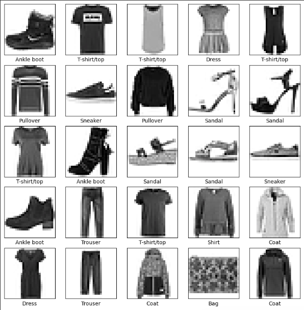
We build the mode after configuring the layers. The basic building block of a neural network is the layer. Layers extract representations from the data fed into them. Hopefully, these representations are meaningful for the problem at hand.
Most of the deep learning consists of chaining together simple layers. Most layers, such as tf.keras.layers.Dense, have parameters that are learned during training.
model = keras.Sequential([
    keras.layers.Flatten(input_shape=(28, 28)),
    keras.layers.Dense(128, activation='relu'),
    keras.layers.Dense(10)
])
The first layer in this network, tf.keras.layers.Flatten, transforms the format of the images from a two-dimensional array (of 28 by 28 pixels) to a one-dimensional array (of 28 * 28 = 784 pixels). Think of this layer as unstacking rows of pixels in the image and lining them up. This layer has no parameters to learn; it only reformats the data.
After the pixels are flattened, the network consists of a sequence of two tf.keras.layers.Dense layers. These are densely connected, or fully connected, neural layers. The first Dense layer has 128 nodes (or neurons). The second (and last) layer returns a logits array with a length of 10. Each node contains a score that indicates the current image belongs to one of the 10 classes.
We then compile the model just like we did in the first use case, but with different parameters.
model.compile(optimizer='adam',
              loss=tf.keras.losses.SparseCategoricalCrossentropy(from_logits=True),
              metrics=['accuracy'])
Then, we feed the model using the model.fit function. We call the fit function as it fits the model to the given dataset.
model.fit(train_images, train_labels, epochs=10)Now, we need to verify the accuracy of our model by using the 10000 images that we kept aside initially.
test_loss, test_acc = model.evaluate(test_images,  test_labels, verbose=2)

print('\nTest accuracy:', test_acc)
The output of the above code is : 313/313 - 1s - loss: 0.3321 - accuracy: 0.8836 - 956ms/epoch - 3ms/step Test accuracy: 0.8835999965667725
This means that our model can predict the output with 88.3599% accuracy.
Use case 3 - Rock paper scissor
We use TensorFlow for image classification in a rock paper and scissors game. You can access the code on Google Colab.
We start by downloading the images required for training the model. We do this by running the following script.
!wget --no-check-certificate \
    https://storage.googleapis.com/laurencemoroney-blog.appspot.com/rps.zip \
    -O /tmp/rps.zip

!wget --no-check-certificate \
    https://storage.googleapis.com/laurencemoroney-blog.appspot.com/rps-test-set.zip \
    -O /tmp/rps-test-set.zip
Since the download files will be in a zip format, we'll use the zipfile library to unzip the files by running the following script.
import os
import zipfile

local_zip = '/tmp/rps.zip'
zip_ref = zipfile.ZipFile(local_zip, 'r')
zip_ref.extractall('/tmp/')
zip_ref.close()

local_zip = '/tmp/rps-test-set.zip'
zip_ref = zipfile.ZipFile(local_zip, 'r')
zip_ref.extractall('/tmp/')
zip_ref.close()
We then use the os library to join the files and put them in a certain directory.
rock_dir = os.path.join('/tmp/rps/rock')
paper_dir = os.path.join('/tmp/rps/paper')
scissors_dir = os.path.join('/tmp/rps/scissors')

print('total training rock images:', len(os.listdir(rock_dir)))
print('total training paper images:', len(os.listdir(paper_dir)))
print('total training scissors images:', len(os.listdir(scissors_dir)))

rock_files = os.listdir(rock_dir)
print(rock_files[:10])

paper_files = os.listdir(paper_dir)
print(paper_files[:10])

scissors_files = os.listdir(scissors_dir)
print(scissors_files[:10])
Now since we don't have labels for this dataset, we put the sample images in respective directories as given in the above code which will generate the labels for us. This is done using ImageDataGenerator library.
%matplotlib inline

import matplotlib.pyplot as plt
import matplotlib.image as mpimg

pic_index = 2

next_rock = [os.path.join(rock_dir, fname)
                for fname in rock_files[pic_index-2:pic_index]]
next_paper = [os.path.join(paper_dir, fname)
                for fname in paper_files[pic_index-2:pic_index]]
next_scissors = [os.path.join(scissors_dir, fname)
                for fname in scissors_files[pic_index-2:pic_index]]

for i, img_path in enumerate(next_rock+next_paper+next_scissors):
  #print(img_path)
  img = mpimg.imread(img_path)
  plt.imshow(img)
  plt.axis('Off')
  plt.show()
We then make and compile the model by the following code
import tensorflow as tf
import keras_preprocessing
from keras_preprocessing import image
from keras_preprocessing.image import ImageDataGenerator

TRAINING_DIR = "/tmp/rps/"
training_datagen = ImageDataGenerator(
      rescale = 1./255,
	    rotation_range=40,
      width_shift_range=0.2,
      height_shift_range=0.2,
      shear_range=0.2,
      zoom_range=0.2,
      horizontal_flip=True,
      fill_mode='nearest')

VALIDATION_DIR = "/tmp/rps-test-set/"
validation_datagen = ImageDataGenerator(rescale = 1./255)

train_generator = training_datagen.flow_from_directory(
	TRAINING_DIR,
	target_size=(150,150),
	class_mode='categorical',
  batch_size=126
)

validation_generator = validation_datagen.flow_from_directory(
	VALIDATION_DIR,
	target_size=(150,150),
	class_mode='categorical',
  batch_size=126
)

model = tf.keras.models.Sequential([
    # Note the input shape is the desired size of the image 150x150 with 3 bytes color
    # This is the first convolution
    tf.keras.layers.Conv2D(64, (3,3), activation='relu', input_shape=(150, 150, 3)),
    tf.keras.layers.MaxPooling2D(2, 2),
    # The second convolution
    tf.keras.layers.Conv2D(64, (3,3), activation='relu'),
    tf.keras.layers.MaxPooling2D(2,2),
    # The third convolution
    tf.keras.layers.Conv2D(128, (3,3), activation='relu'),
    tf.keras.layers.MaxPooling2D(2,2),
    # The fourth convolution
    tf.keras.layers.Conv2D(128, (3,3), activation='relu'),
    tf.keras.layers.MaxPooling2D(2,2),
    # Flatten the results to feed into a DNN
    tf.keras.layers.Flatten(),
    tf.keras.layers.Dropout(0.5),
    # 512 neuron hidden layer
    tf.keras.layers.Dense(512, activation='relu'),
    tf.keras.layers.Dense(3, activation='softmax')
])


model.summary()

model.compile(loss = 'categorical_crossentropy', optimizer='rmsprop', metrics=['accuracy'])

history = model.fit(train_generator, epochs=25, steps_per_epoch=20, validation_data = validation_generator, verbose = 1, validation_steps=3)

model.save("rps.h5")
We just execute the above code just like we did in the previous 2 use cases.
This takes us to the end of this transcript blog. This was just a basic overview of deep learning using TensorFlow. To understand more, you can check out the official TensorFlow documentation here.
Questions and answers
- Why didn't we use
averagepooling layer instead ofmax?
This is just one use case and average pooling layer can also be tried out instead of max. The average layer is also known to have more accuracy. Since this is just a very basic example, it doesn't make much difference which layer we use. There are more concepts that weren't covered in the session.
2. How to decide which loss function to use?
It depends on the usecase. You can go to keras.io which is the official documentation to learn more and understand the ABCD of ML. All the details and use cases of the loss function are present in the keras official documentation.
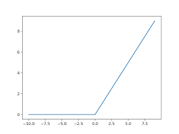
3. Why do we use relu activation function?
For every output less than 0, relu considers it to be 0 itself. There are other activation functions like softmax. It will also give us a value between 0 and 1. This is because we don't label the value other than 0 to 1.
4. How to decide how many deep layers to use?
There is no hard and fast rule to decide this. To understand this better, you can go to the TensorFlow hub and learn more there.
Conclusion
This was the final message by the speaker. Get started right away and don't get overwhelmed by new terminologies. Take the first step and you'll automatically get it. There are people who were able to get silver and bronze medals with just one month of learning. So don't think you can't do it.
For more such talks, attend Git Commit Show live. The next season is coming soon!


Member discussion